The core implementation — installing MTEB, loading the model, running evaluation on Banking77 — reproduces the paper's methodology. The results (~67% accuracy) validate what the paper reported for this model class. Our original contribution is the visualisation function: three separate subplots tracking Accuracy, F1, and Weighted F1 across all 10 experiments. The original paper outputs raw JSON only. We wrote the code to make those results readable and analysable across runs. That's a small but real addition — and I'd rather be clear about the distinction than oversell it.
What is MTEB?
Before MTEB, evaluating text embeddings was fragmented. Different papers used different tasks, different metrics, different datasets — making it nearly impossible to know whether one model was genuinely better than another, or just better on the specific benchmark its authors chose to highlight.
The Massive Text Embedding Benchmark, published in 2022, fixes this by providing a unified evaluation framework across 58 datasets, 112 languages, and 8 task categories — classification, clustering, retrieval, semantic similarity, and more. The value is standardisation: run your model on MTEB once and your score is directly comparable to every other model on the leaderboard.
Why this benchmarking problem matters
Earlier frameworks each solved a slice of the problem. SuperGLUE evaluated natural language understanding but had limited scope. BEIR covered retrieval but nothing else. SBERT-based evaluations were expensive and narrow. None gave a complete picture of how an embedding model actually performs across the range of tasks it would encounter in practice.
| Benchmark | Focus | Limitation |
|---|---|---|
| SuperGLUE | NLU tasks | Limited scope |
| BEIR | Retrieval only | Not general purpose |
| SBERT | Sentence similarity | Narrow and expensive |
| MTEB | All embedding tasks | Still being adopted at time of writing |
The model — and why it's a useful baseline
We used average_word_embeddings_komninos — a model that represents a sentence by averaging its individual word vectors. There's no attention, no context window, no transformer architecture. "Bank" as a financial institution and "bank" as a riverbank produce the same vector regardless of surrounding words.
That's exactly why it makes a useful starting point. Word-averaging embeddings are lightweight and stable, but they have a ceiling that contextual models like BERT were built to break through. Establishing that ceiling is the first step in meaningful model comparison — which is what MTEB is designed to enable.
Implementation — the reproduction
!pip install mteb sentence-transformers

from huggingface_hub import login
login(token='YOUR_HF_TOKEN')  # required to access model hub
import mteb
from sentence_transformers import SentenceTransformer

model_name = "average_word_embeddings_komninos"
model      = SentenceTransformer(model_name)

# Banking77: intent classification across 77 banking query categories
tasks      = mteb.get_tasks(tasks=["Banking77Classification"])
evaluation = mteb.MTEB(tasks=tasks)
results    = evaluation.run(model, output_folder=f"results/{model_name}")
import json

with open('results/.../Banking77Classification.json', 'r') as file:
    results_data = json.load(file)

print(f"Overall Accuracy:     {results_data['scores']['test'][0]['accuracy']:.2f}")
print(f"Overall F1:           {results_data['scores']['test'][0]['f1']:.2f}")
print(f"Overall Weighted F1:  {results_data['scores']['test'][0]['f1_weighted']:.2f}")
Our contribution — the visualisation function
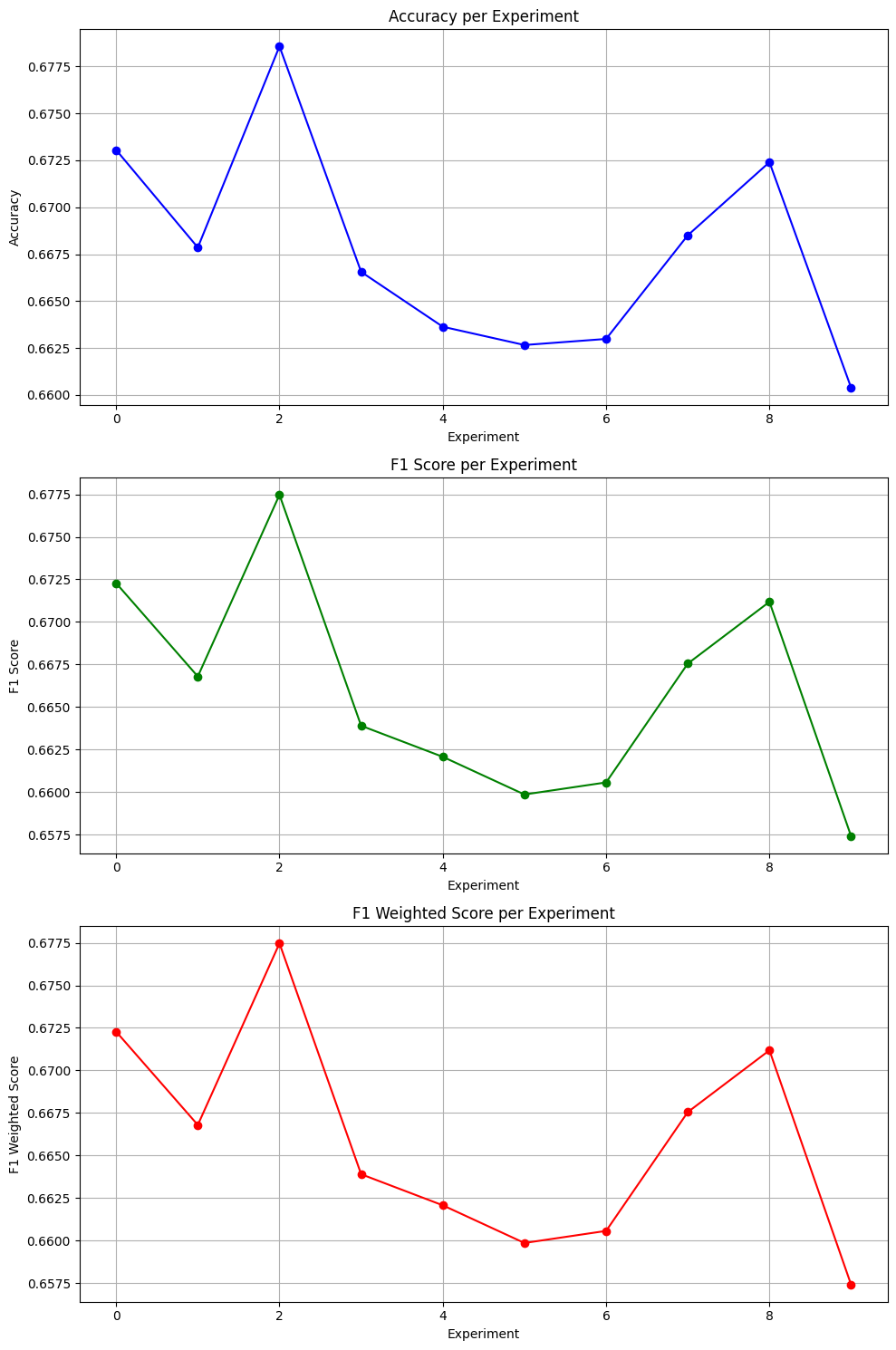
The paper's output is raw JSON — useful for pipelines, but hard to read across multiple experiments. We wrote a three-panel visualisation function that plots Accuracy, F1, and Weighted F1 separately across all 10 experiment runs, making variance and patterns immediately visible rather than requiring you to scan through numbers.
import matplotlib.pyplot as plt

def visualize_test_scores(test_scores):
    experiments     = test_scores[0]['scores_per_experiment']

    accuracy_scores = [e['accuracy']   for e in experiments]
    f1_scores       = [e['f1']         for e in experiments]
    f1_weighted     = [e['f1_weighted'] for e in experiments]

    fig, axes = plt.subplots(3, 1, figsize=(10, 15))

    axes[0].plot(accuracy_scores, marker='o', color='b')
    axes[0].set_title('Accuracy per Experiment')
    axes[0].set_xlabel('Experiment')
    axes[0].set_ylabel('Accuracy')
    axes[0].grid(True)

    axes[1].plot(f1_scores, marker='o', color='g')
    axes[1].set_title('F1 Score per Experiment')
    axes[1].set_xlabel('Experiment')
    axes[1].set_ylabel('F1 Score')
    axes[1].grid(True)

    axes[2].plot(f1_weighted, marker='o', color='r')
    axes[2].set_title('F1 Weighted Score per Experiment')
    axes[2].set_xlabel('Experiment')
    axes[2].set_ylabel('F1 Weighted Score')
    axes[2].grid(True)

    plt.tight_layout()
    plt.show()

visualize_test_scores(results_data["scores"]["test"])
Results
| Experiment | Accuracy | F1 | Weighted F1 |
|---|---|---|---|
| 1 | 0.67 | 0.67 | 0.67 |
| 2 | 0.67 | 0.67 | 0.67 |
| 3 | 0.68 | 0.68 | 0.68 |
| 4 | 0.67 | 0.66 | 0.66 |
| 5 | 0.66 | 0.66 | 0.66 |
| 6 | 0.66 | 0.66 | 0.66 |
| 7 | 0.66 | 0.66 | 0.66 |
| 8 | 0.67 | 0.67 | 0.67 |
| 9 | 0.67 | 0.67 | 0.67 |
| 10 | 0.66 | 0.66 | 0.66 |
What the results actually tell us
Three things stand out. First, Accuracy, F1, and Weighted F1 track almost identically across all 10 runs — a sign of balanced class handling. The model isn't favouring any particular intent category over others across 77 classes, which is a meaningful property to confirm.
Second, the variance is small — just 0.02 between best and worst experiment. That confirms the reproduction is stable and the setup is correct.
Third, the dip across experiments 5–7 before recovering is the most interesting pattern in the charts. A static word-embedding model has no mechanism to adapt between runs — it's deterministic given the same inputs. The variability comes from how the dataset is split and shuffled across experiments, not from the model itself. That's a useful thing to understand about what you're measuring.
67% on a 77-class classification task without any contextual understanding is a reasonable baseline. A transformer-based model like all-MiniLM-L6-v2 would push this well above 80% — running that comparison is the obvious next step.
Limitations
We ran this on a single task with a single model. That's enough to validate the framework and understand the baseline, but not enough to draw broader conclusions about MTEB or embedding models generally. We didn't run any model comparisons, didn't tune anything (word-averaging models have no hyperparameters to tune), and didn't add a confusion matrix across the 77 intent categories — which is where the more interesting analysis would start.
References
- MTEB paper: arxiv.org/pdf/2210.07316v3
- MTEB GitHub: github.com/embeddings-benchmark/mteb